Understanding Batch Normalization
I took Andrew’s Deep Learning course on Coursera, the course teaches you how to effectively design a neural network from scratch. It was extremely useful in my understanding of what is happening behind the scene. The bottom-up approach of the course makes it really interesting. The way Andrew breaks down some of these seemly complex techniques and algorithms in the course is joy to watch. From batch normalisation to mini-batch gradient descent to hyperparameters tuning.
That being said, let us get down to the business we have in hand today. Implementing batch normalization! In our previous post where we looked at implementing neural network from scratch. The first thing we did was to pre-processed our data. That was normalization. We understood that normalizing the input features can speed up learnings. What we did was to compute the mean, the variances and then normalized the data according to the variances.

As we saw in the post, normalizing the input can turn the contours of our learning problem from a very elongated shape to something very more rounded which makes it easier for our gradient descent algorithm to optimize.

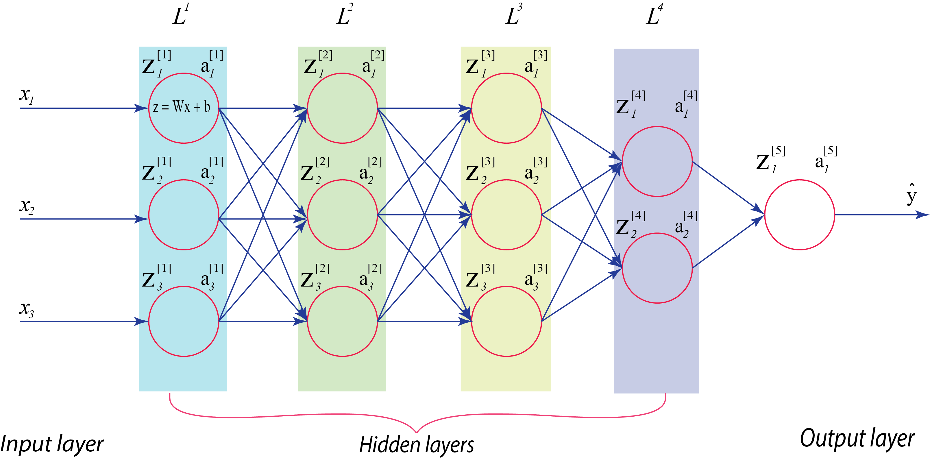
Now for a deeper model where we have the input features and several hidden activation layers in our network, and we want to normalize the hidden layers and not just the input features of our model. It would be nice to normalize the mean and variances of the activation function of the previous layer. This will make the training of our paramters more efficient.
For any hidden layer, we can normalize the value of say in hidden layer so as to train the values of faster and make our model more efficient.
Considering our deep learning example from the perspective of a certain layer, say the 4th hidden layer, . So our network has to learn the parameters . From the perspective of this 4th hidden layer, each of the preceeding layers have great influence over what the input of this layer will see. As you start to train your network, the distribution of what this layer sees will vary significantly with time. As an analogy, let us say you train your dataset on all images of black cats, if you try to apply this same network to dataset with coloured cats where the positive examples are not just black cats, then your classifier or prediction will perform poorly. This concept where the training dataset distribution is different from the text dataset distribution is known as . The idea is that if you’ve learned some to mapping, , and at any time the distribution of changes, then you might need to retrain your learning algorithm.
So what batch norm does is to reduce the the amount that the distribution of the hidden units shift around. No matter how the parameter of the previous layer changes, their mean and variance will remain thesame. It limits the amount to which updating the parameters of the earlier layers can affect the distribution of values that the current layer now sees and therefore has to learn on. This makes the values of the current layer to become more stable and provide the later layers more firm ground to stand on. Another interesting thing about batch norm is that it has a slight regularization effect. Though this is really not the intent of batch norm but sometimes it has this intended or unintended effect on your learning algorithm.
Implementing Batch Normalization
Given some intermediate values in a neural network, we can add batch norm by first, feeding the input into the first hidden layer and then compute govern by the parameters . We then take this parameter and apply batch norm govern by the parameters and . This will give us the new normalized value , which we then feed into the activation function to give us .
Now we’ve done the computation for the first hidden layer . Next, we take the value and use it to compute the batch norm for the next hidden layer and so on.
With these new set of parameters in our algorithm, we can then use whatever optimization technique we want to. So far, we’ve been talking about batch norm as if we were training on the entire training set at thesame time, like we’re using batch gradient descent. However, It is worth noting that in practice, batch normalization is usually applied with mini-batches in training set.
for t = 1 ... n(mini-batches)
  compute forward propagation on X{t}
	in each hidden layer, use BN to replace Z[l] with z^[l]
  compute  dW[l], dbeta, dgamma using backward propagation

  update parameters dW[l] := dW[l] - alpha.dW[l]
		    dbeta := dbeta - alpha.dbeta
		    dgamma:= dgamma- alpha.dgamma
end
Also checking out this maths function witk LateX:
Check out the Jekyll docs for more info on how to get the most out of Jekyll. File all bugs/feature requests at Jekyll’s GitHub repo. If you have questions, you can ask them on Jekyll Talk.
